Inference for Comparing Two Paired Means/ Comparing Multiple Means with ANOVA

Author

Sara S

library(tidyverse)
── Attaching core tidyverse packages ──────────────────────── tidyverse 2.0.0 ──
✔ dplyr     1.1.4     ✔ readr     2.1.5
✔ forcats   1.0.0     ✔ stringr   1.5.1
✔ ggplot2   3.5.1     ✔ tibble    3.2.1
✔ lubridate 1.9.3     ✔ tidyr     1.3.1
✔ purrr     1.0.2     
── Conflicts ────────────────────────────────────────── tidyverse_conflicts() ──
✖ dplyr::filter() masks stats::filter()
✖ dplyr::lag()    masks stats::lag()
ℹ Use the conflicted package (<http://conflicted.r-lib.org/>) to force all conflicts to become errors
library(mosaic)
Registered S3 method overwritten by 'mosaic':
  method                           from   
  fortify.SpatialPolygonsDataFrame ggplot2

The 'mosaic' package masks several functions from core packages in order to add 
additional features.  The original behavior of these functions should not be affected by this.

Attaching package: 'mosaic'

The following object is masked from 'package:Matrix':

    mean

The following objects are masked from 'package:dplyr':

    count, do, tally

The following object is masked from 'package:purrr':

    cross

The following object is masked from 'package:ggplot2':

    stat

The following objects are masked from 'package:stats':

    binom.test, cor, cor.test, cov, fivenum, IQR, median, prop.test,
    quantile, sd, t.test, var

The following objects are masked from 'package:base':

    max, mean, min, prod, range, sample, sum
library(broom) # Tidy Test data
library(resampledata3) # Datasets from Chihara and Hesterberg's book

Attaching package: 'resampledata3'

The following object is masked from 'package:datasets':

    Titanic
library(gt) # for tables
library(infer) # Statistical Inference, Permutation/Bootstrap

Attaching package: 'infer'

The following objects are masked from 'package:mosaic':

    prop_test, t_test
library(patchwork) # Arranging Plots
library(ggprism) # Interesting Categorical Axes
library(supernova) # Beginner-Friendly ANOVA Tables

Reading the Dataset

frogs_orig <- read_csv("../../data/frogs.csv")
Rows: 60 Columns: 4
── Column specification ────────────────────────────────────────────────────────
Delimiter: ","
dbl (4): Frogspawn sample id, Temperature13, Temperature18, Temperature25

ℹ Use `spec()` to retrieve the full column specification for this data.
ℹ Specify the column types or set `show_col_types = FALSE` to quiet this message.
frogs_orig
# A tibble: 60 × 4
   `Frogspawn sample id` Temperature13 Temperature18 Temperature25
                   <dbl>         <dbl>         <dbl>         <dbl>
 1                     1            24            NA            NA
 2                     2            NA            21            NA
 3                     3            NA            NA            18
 4                     4            26            NA            NA
 5                     5            NA            22            NA
 6                     6            NA            NA            14
 7                     7            27            NA            NA
 8                     8            NA            22            NA
 9                     9            NA            NA            15
10                    10            27            NA            NA
# ℹ 50 more rows

Clean the Data

frogs_orig %>%
  pivot_longer(
    .,
    cols = starts_with("Temperature"),
    cols_vary = "fastest",
    # new in pivot_longer
    names_to = "Temp",
    values_to = "Time"
  ) %>%
  drop_na() %>%
  ##
  separate_wider_regex(
    cols = Temp,
    # knock off the unnecessary "Temperature" word
    # Just keep the digits thereafter
    patterns = c("Temperature", TempFac = "\\d+"),
    cols_remove = TRUE
  ) %>%
  # Convert Temp into TempFac, a 3-level factor
  mutate(TempFac = factor(
    x = TempFac,
    levels = c(13, 18, 25),
    labels = c("13", "18", "25")
  )) %>%
  rename("Id" = `Frogspawn sample id`) -> frogs_long
frogs_long
# A tibble: 60 × 3
      Id TempFac  Time
   <dbl> <fct>   <dbl>
 1     1 13         24
 2     2 18         21
 3     3 25         18
 4     4 13         26
 5     5 18         22
 6     6 25         14
 7     7 13         27
 8     8 18         22
 9     9 25         15
10    10 13         27
# ℹ 50 more rows
##
frogs_long %>% count(TempFac)
# A tibble: 3 × 2
  TempFac     n
  <fct>   <int>
1 13         20
2 18         20
3 25         20

Workflow for Exploratory Data Analysis (EDA)

gf_histogram(~Time,
  fill = ~TempFac,
  data = frogs_long, alpha = 0.5
) %>%
  gf_vline(xintercept = ~ mean(Time)) %>%
  gf_labs(
    title = "Histograms of Hatching Time Distributions vs Temperature",
    x = "Hatching Time", y = "Count"
  ) %>%
  gf_text(7 ~ (mean(Time) + 2),
    label = "Overall Mean"
  ) %>%
  gf_refine(guides(fill = guide_legend(title = "Temperature level (°C)")))

gf_boxplot(
  data = frogs_long,
  Time ~ TempFac,
  fill = ~TempFac,
  alpha = 0.5
) %>%
  gf_vline(xintercept = ~ mean(Time)) %>%
  gf_labs(
    title = "Boxplots of Hatching Time Distributions vs Temperature",
    x = "Temperature", y = "Hatching Time",
    caption = "Using ggprism"
  ) %>%
  gf_refine(
    scale_x_discrete(guide = "prism_bracket"),
    guides(fill = guide_legend(title = "Temperature level (°C)"))
  )
Warning: The S3 guide system was deprecated in ggplot2 3.5.0.
ℹ It has been replaced by a ggproto system that can be extended.

ANOVA

frogs_anova <- aov(Time ~ TempFac, data = frogs_long)
supernova::pairwise(frogs_anova,
  correction = "Bonferroni", # Try "Tukey"
  alpha = 0.05, # 95% CI calculation
  var_equal = TRUE, # We'll see
  plot = TRUE
)

── Pairwise t-tests with Bonferroni correction ─────────────────────────────────
Model: Time ~ TempFac
TempFac
Levels: 3
Family-wise error-rate: 0.049

  group_1 group_2    diff pooled_se       t    df   lower  upper p_adj
  <chr>   <chr>     <dbl>     <dbl>   <dbl> <int>   <dbl>  <dbl> <dbl>
1 18      13       -5.300     0.257 -20.608    57  -5.861 -4.739 .0000
2 25      13      -10.100     0.257 -39.272    57 -10.661 -9.539 .0000
3 25      18       -4.800     0.257 -18.664    57  -5.361 -4.239 .0000

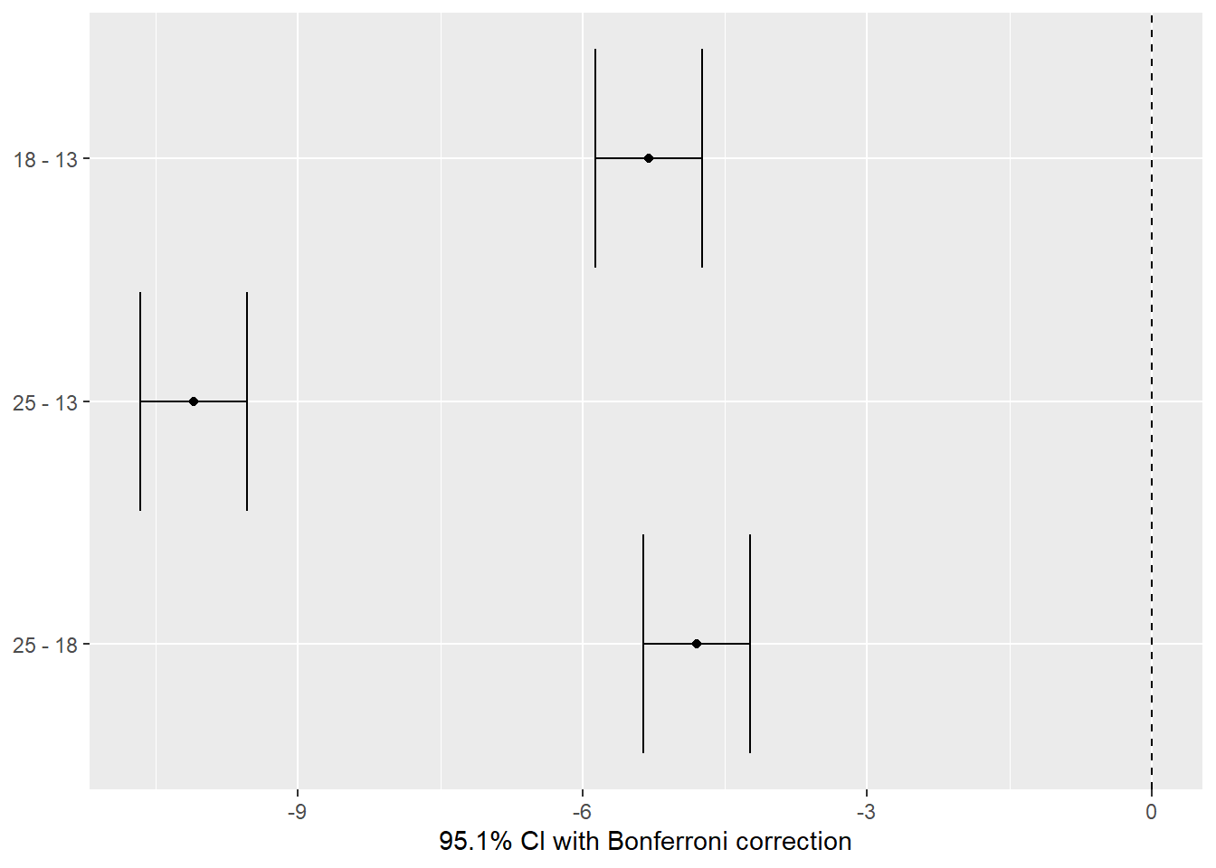
the black points are the difference in the means of the hatching time. yaxis the groups pairwise xaxis difference in means of the groups the lines are the confidence intervals pairwise

variants is square of all the numbers

total sum of squares sst monster number individual number

sse error sum of squares