Groups

Author

Sara S

Installing packages

library(tidyverse)
── Attaching core tidyverse packages ──────────────────────── tidyverse 2.0.0 ──
✔ dplyr     1.1.4     ✔ readr     2.1.5
✔ forcats   1.0.0     ✔ stringr   1.5.1
✔ ggplot2   3.5.1     ✔ tibble    3.2.1
✔ lubridate 1.9.3     ✔ tidyr     1.3.1
✔ purrr     1.0.2     
── Conflicts ────────────────────────────────────────── tidyverse_conflicts() ──
✖ dplyr::filter() masks stats::filter()
✖ dplyr::lag()    masks stats::lag()
ℹ Use the conflicted package (<http://conflicted.r-lib.org/>) to force all conflicts to become errors
library(mosaic)
Registered S3 method overwritten by 'mosaic':
  method                           from   
  fortify.SpatialPolygonsDataFrame ggplot2

The 'mosaic' package masks several functions from core packages in order to add 
additional features.  The original behavior of these functions should not be affected by this.

Attaching package: 'mosaic'

The following object is masked from 'package:Matrix':

    mean

The following objects are masked from 'package:dplyr':

    count, do, tally

The following object is masked from 'package:purrr':

    cross

The following object is masked from 'package:ggplot2':

    stat

The following objects are masked from 'package:stats':

    binom.test, cor, cor.test, cov, fivenum, IQR, median, prop.test,
    quantile, sd, t.test, var

The following objects are masked from 'package:base':

    max, mean, min, prod, range, sample, sum
library(ggformula)
library(skimr)

Attaching package: 'skimr'

The following object is masked from 'package:mosaic':

    n_missing
library(palmerpenguins)

Dataset: Wages

wages <- read.csv("https://vincentarelbundock.github.io/Rdatasets/csv/stevedata/gss_wages.csv")

Organizing the data

glimpse(wages)
Rows: 61,697
Columns: 12
$ rownames   <int> 1, 2, 3, 4, 5, 6, 7, 8, 9, 10, 11, 12, 13, 14, 15, 16, 17, …
$ year       <int> 1974, 1974, 1974, 1974, 1974, 1974, 1974, 1974, 1974, 1974,…
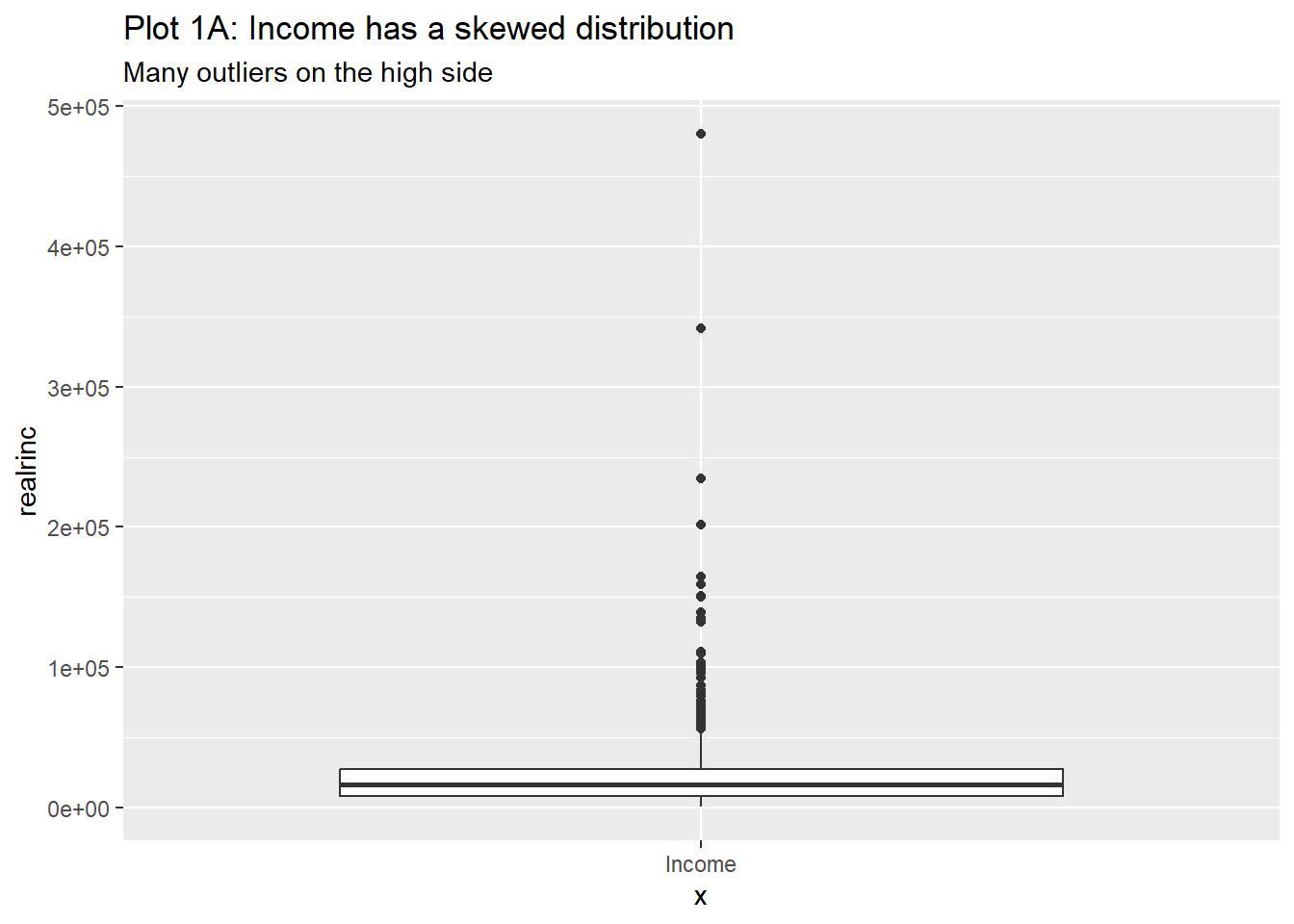
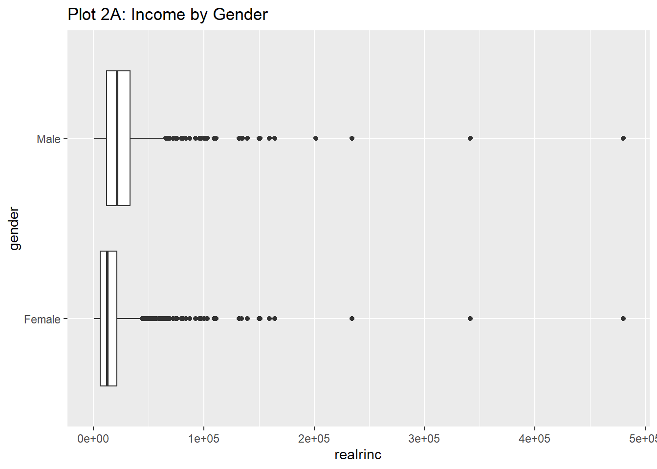
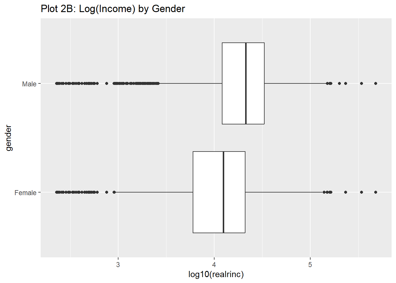
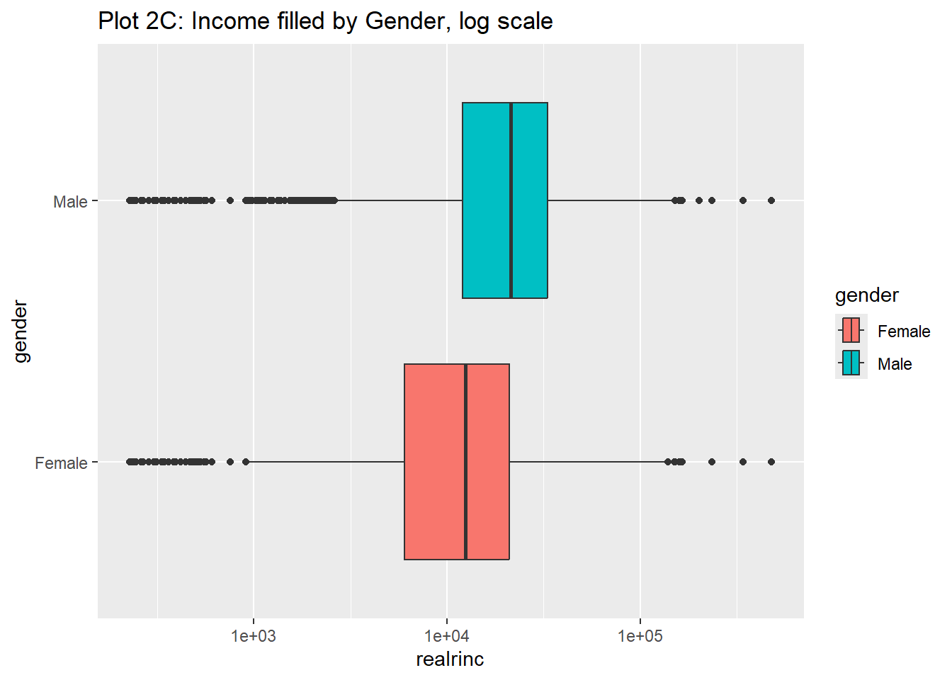
$ realrinc   <dbl> 4935, 43178, NA, NA, 18505, 22206, 55515, NA, NA, 4935, NA,…
$ age        <int> 21, 41, 83, 69, 58, 30, 48, 67, 51, 54, 89, 71, 27, 30, 22,…
$ occ10      <int> 5620, 2040, NA, NA, 5820, 910, 230, 6355, 4720, 3940, 4810,…
$ occrecode  <chr> "Office and Administrative Support", "Professional", "", ""…
$ prestg10   <int> 25, 66, NA, NA, 37, 45, 59, 49, 28, 38, 47, 45, 50, 29, 33,…
$ childs     <int> 0, 3, 2, 2, 0, 0, 2, 1, 2, 2, 3, 1, 4, 3, 0, 1, 2, 3, 4, 8,…
$ wrkstat    <chr> "School", "Full-Time", "Housekeeper", "Housekeeper", "Full-…
$ gender     <chr> "Male", "Male", "Female", "Female", "Female", "Male", "Male…
$ educcat    <chr> "High School", "Bachelor", "Less Than High School", "Less T…
$ maritalcat <chr> "Married", "Married", "Widowed", "Widowed", "Never Married"…
inspect(wages)

categorical variables:  
        name     class levels     n missing
1  occrecode character     12 61697       0
2    wrkstat character      9 61697       0
3     gender character      2 61697       0
4    educcat character      6 61697       0
5 maritalcat character      6 61697       0
                                   distribution
1 Professional (17.9%), Service (16%) ...      
2 Full-Time (49.4%), Housekeeper (15.1%) ...   
3 Female (56.1%), Male (43.9%)                 
4 High School (51.4%) ...                      
5 Married (51.7%), Never Married (21.8%) ...   

quantitative variables:  
      name   class  min    Q1 median    Q3      max         mean           sd
1 rownames integer    1 15425  30849 46273  61697.0 30849.000000 17810.534116
2     year integer 1974  1985   1996  2006   2018.0  1996.073715    12.794470
3 realrinc numeric  227  8156  16563 27171 480144.5 22326.359234 28581.794499
4      age integer   18    32     44    59     89.0    46.176177    17.561065
5    occ10 integer   10  2710   4720  6230   9997.0  4695.774081  2627.724076
6 prestg10 integer   16    33     42    50     80.0    43.060701    12.987526
7   childs integer    0     0      2     3      8.0     1.923457     1.763569
      n missing
1 61697       0
2 61697       0
3 37887   23810
4 61478     219
5 58136    3561
6 57511    4186
7 61508     189
skimr:: skim(wages)
Data summary
Name wages
Number of rows 61697
Number of columns 12
_______________________
Column type frequency:
character 5
numeric 7
________________________
Group variables None

Variable type: character

skim_variable n_missing complete_rate min max empty n_unique whitespace
occrecode 0 1 0 37 3561 12 0
wrkstat 0 1 0 23 21 9 0
gender 0 1 4 6 0 2 0
educcat 0 1 0 21 135 6 0
maritalcat 0 1 0 13 27 6 0

Variable type: numeric

skim_variable n_missing complete_rate mean sd p0 p25 p50 p75 p100 hist
rownames 0 1.00 30849.00 17810.53 1 15425 30849 46273 61697.0 ▇▇▇▇▇
year 0 1.00 1996.07 12.79 1974 1985 1996 2006 2018.0 ▆▇▇▇▇
realrinc 23810 0.61 22326.36 28581.79 227 8156 16563 27171 480144.5 ▇▁▁▁▁
age 219 1.00 46.18 17.56 18 32 44 59 89.0 ▇▇▆▅▂
occ10 3561 0.94 4695.77 2627.72 10 2710 4720 6230 9997.0 ▃▅▇▂▃
prestg10 4186 0.93 43.06 12.99 16 33 42 50 80.0 ▃▇▇▃▁
childs 189 1.00 1.92 1.76 0 0 2 3 8.0 ▇▇▂▁▁

Dropping the missing values

wages_clean <-
  wages %>%
  tidyr::drop_na(realrinc) 

Distribution of realrinc

Notes: Properties of boxplot are as follows-

  • Median (Middle Line in the Box): The line inside the box represents the median, dividing the data into two halves.

  • Interquartile Range (IQR): The box spans from the first quartile (Q1, 25th percentile) to the third quartile (Q3, 75th percentile), covering the middle 50% of the data.

  • Whiskers: These extend from Q1 down to the minimum and from Q3 up to the maximum values, but only within 1.5 times the IQR. Data beyond this range are considered outliers.

  • Outliers: Data points outside the whiskers are shown as individual points or small markers, indicating they are significantly different from the rest of the data.

  • Symmetry/Skewness: If the box is centered and the whiskers are balanced, the data is symmetric. If not, the data is skewed (longer whisker shows skew direction).

wages_clean %>%
  gf_boxplot(realrinc ~ "Income") %>% # Dummy X-axis "variable"
  gf_labs(
    title = "Plot 1A: Income has a skewed distribution",
    subtitle = "Many outliers on the high side"
  )

This box plot displays the distribution of realrinc (real income) overall. Since there is a skew in the data, with a tail on the higher end, many high-income outliers are shown. The box plot will have a longer whisker towards the high-income values, and many points beyond the whiskers, indicating those outliers.

Is realrinc affected by gender?

wages_clean %>%
  gf_boxplot(gender ~ realrinc) %>%
  gf_labs(title = "Plot 2A: Income by Gender")

Comparing income by gender shows a noticeable difference between the two groups. The median income for males is higher than for females, and the distribution for males tends to have more variation, with a broader spread and more outliers. This shows a gender income gap, with males generally earning more than females.

Is a logged realrinc affected by gender?

wages_clean %>%
  gf_boxplot(gender ~ log10(realrinc)) %>%
  gf_labs(title = "Plot 2B: Log(Income) by Gender")

Logging the income data ‘log10(realrinc)’ and plotting it by gender makes the income distribution less skewed and easier to interpret. The log transformation helps to compress the extreme values.

Is realrinc affected by gender when x-axis is logged?

wages_clean %>%
  gf_boxplot(gender ~ realrinc, fill = ~gender) %>%
  gf_refine(scale_x_log10()) %>%
  gf_labs(title = "Plot 2C: Income filled by Gender, log scale")

When applying a log scale to the x-axis, income is still higher for males than females. The fill colors differentiate between genders, and the log scale brings out the differences more clearly.

Is realrinc affected by education (educcat)?

wages_clean %>%
  gf_boxplot(educcat ~ realrinc) %>%
  gf_labs(title = "Plot 3A: Income by Education Category")

Income distribution by education level shows that people with higher education usually earn more. There is a lot of variation within each education group, and some highly educated individuals (graduates and bachelors) earn much more than most others in their category.

Is logged realrinc affected by education (educcat)?

wages_clean %>%
  gf_boxplot(educcat ~ log10(realrinc)) %>%
  gf_labs(title = "Plot 3B: Log(Income) by Education Category")

After applying a log transformation, the differences between education categories become clearer, and the skewness of income distributions is reduced. The higher the education level, the higher the income is and the differences between categories are more easily comparable due to the log scale.

Is realrinc affected by education (educcat) when reorder education is reordered based on the median of realrinc?

wages_clean %>%
  gf_boxplot(
    reorder(educcat, realrinc, FUN = median) ~ log(realrinc),
    fill = ~educcat,
    alpha = 0.3
  ) %>%
  gf_labs(title = "Plot 3C: Log(Income) by Education Category, sorted") %>%
  gf_labs(
    x = "Log Income",
    y = "Education Category"
  )

By reordering the education categories based on the median income, the plot more clearly shows the increasing in income as education levels rise.

realrinc by education sorted by median of realrinc with a logged x-axis

Notes: ‘FUN = median’ tells R to apply the median function to a group of values, calculating the middle value of each subset, often used for summarizing or sorting data based on average. FUN stands for function, and this function can be used for calculations like mean, sum, and more.

wages_clean %>%
  gf_boxplot(reorder(educcat, realrinc, FUN = median) ~ realrinc,
    fill = ~educcat,
    alpha = 0.5
  ) %>%
  gf_refine(scale_x_log10()) %>%
  gf_labs(
    title = "Plot 3D: Income by Education Category, sorted",
    subtitle = "Log Income"
  ) %>%
  gf_labs(
    x = "Income",
    y = "Education Category"
  )

Since the education categories sorted and the income axis logged, the income spread looks more balanced, making it easier to compare different education levels.

Is realrinc affected by combinations of factors like gender, education, marital status and number of children?

wages %>%
  drop_na() %>%
  gf_boxplot(reorder(educcat, realrinc) ~ log10(realrinc),
    fill = ~educcat,
    alpha = 0.5
  ) %>%
  gf_facet_wrap(vars(childs)) %>%
  gf_refine(scale_fill_brewer(type = "qual", palette = "Dark2")) %>%
  gf_labs(
    title = "Plot 4A: Log Income by Education Category and Family Size",
    x = "Log income",
    y = "No. of Children"
  )

Individuals with more children tend to have slightly different income patterns, but education still plays a important role. The faceting by number of children shows how family size interacts with education to affect income levels.

Logged realrinc by number of children facetted by gender

wages %>%
  drop_na() %>%
  mutate(childs = as_factor(childs)) %>%
  gf_boxplot(childs ~ log10(realrinc),
    group = ~childs,
    fill = ~childs,
    alpha = 0.5
  ) %>%
  gf_facet_wrap(~gender) %>%
  gf_refine(scale_fill_brewer(type = "qual", palette = "Set3")) %>%
  gf_labs(
    title = "Plot 4B: Log Income by Gender and Family Size",
    x = "Log income",
    y = "No. of Children"
  )

Males tend to have higher incomes regardless of family size, but the differences between family sizes vary slightly by gender. This shows that while income is influenced by both gender and family size, gender plays a more important role.

Logged realrinc by gender facetted by number of children

wages %>%
  drop_na() %>%
  mutate(childs = as_factor(childs)) %>%
  gf_boxplot(gender ~ log10(realrinc),
    group = ~gender,
    fill = ~gender,
    alpha = 0.5
  ) %>%
  gf_facet_wrap(~childs) %>%
  gf_refine(scale_fill_brewer(type = "qual", palette = "Set3")) %>%
  gf_labs(
    title = "Plot 4C: Log Income by Gender and Family Size",
    x = "Log income",
    y = "No. of Children"
  )

In this plot, gender and income are analyzed using a log10 scale, faceted by the number of children. It highlights that males earn more than females across all family sizes, highlighting gender differences.

Logged realrinc by gender facetted by education

wages %>%
  drop_na() %>%
  mutate(childs = as_factor(childs)) %>%
  gf_boxplot(gender ~ log10(realrinc),
    group = ~gender,
    fill = ~gender,
    alpha = 0.5
  ) %>%
  gf_facet_wrap(~educcat) %>%
  gf_refine(scale_fill_brewer(type = "qual", palette = "Set3")) %>%
  gf_labs(
    title = "Plot 4C: Log Income by Gender and Family Size",
    x = "Log income",
    y = "No. of Children"
  )

Income by gender within each education category shows that even at higher education levels, males tend to earn more than females. Even with higher education, women tend to earn less than men.