The case study named “Chhota Bheem vs Doraemon vs Dragon Tales” is an exploration of difference in ratings for various kids TV shows, scored by student in college.
Importing Packages
library(tidyverse)
── Attaching core tidyverse packages ──────────────────────── tidyverse 2.0.0 ──
✔ dplyr     1.1.4     ✔ readr     2.1.5
✔ forcats   1.0.0     ✔ stringr   1.5.1
✔ ggplot2   3.5.1     ✔ tibble    3.2.1
✔ lubridate 1.9.3     ✔ tidyr     1.3.1
✔ purrr     1.0.2
── Conflicts ────────────────────────────────────────── tidyverse_conflicts() ──
✖ dplyr::filter() masks stats::filter()
✖ dplyr::lag()    masks stats::lag()
ℹ Use the conflicted package (<http://conflicted.r-lib.org/>) to force all conflicts to become errors
library(ggformula)
Loading required package: scales

Attaching package: 'scales'

The following object is masked from 'package:purrr':

    discard

The following object is masked from 'package:readr':

    col_factor

Loading required package: ggridges

New to ggformula?  Try the tutorials:
    learnr::run_tutorial("introduction", package = "ggformula")
    learnr::run_tutorial("refining", package = "ggformula")
library(mosaic)
Registered S3 method overwritten by 'mosaic':
  method                           from
  fortify.SpatialPolygonsDataFrame ggplot2

The 'mosaic' package masks several functions from core packages in order to add
additional features.  The original behavior of these functions should not be affected by this.

Attaching package: 'mosaic'

The following object is masked from 'package:Matrix':

    mean

The following object is masked from 'package:scales':

    rescale

The following objects are masked from 'package:dplyr':

    count, do, tally

The following object is masked from 'package:purrr':

    cross

The following object is masked from 'package:ggplot2':

    stat

The following objects are masked from 'package:stats':

    binom.test, cor, cor.test, cov, fivenum, IQR, median, prop.test,
    quantile, sd, t.test, var

The following objects are masked from 'package:base':

    max, mean, min, prod, range, sample, sum
library(broom)library(infer)
Attaching package: 'infer'

The following objects are masked from 'package:mosaic':

    prop_test, t_test
Attaching package: 'supernova'

The following object is masked from 'package:scales':

    number
library(crosstable)
Attaching package: 'crosstable'

The following object is masked from 'package:purrr':

    compact
Dataset: TV shows
t <-read_csv("../../data/doraemon.csv")
Rows: 90 Columns: 4
── Column specification ────────────────────────────────────────────────────────
Delimiter: ","
chr (3): Participant ID, Gender, Cartoon
dbl (1): Rating

ℹ Use `spec()` to retrieve the full column specification for this data.
ℹ Specify the column types or set `show_col_types = FALSE` to quiet this message.
t
# A tibble: 90 × 4
   `Participant ID` Gender Cartoon     Rating
   <chr>            <chr>  <chr>        <dbl>
 1 P1               Male   Chota Bheem    8.5
 2 P2               Male   Chota Bheem    6
 3 P3               Male   Chota Bheem    8
 4 P4               Male   Chota Bheem    7
 5 P5               Male   Chota Bheem    8
 6 P6               Male   Chota Bheem   10
 7 P7               Male   Chota Bheem    5
 8 P8               Male   Chota Bheem    7.8
 9 P9               Male   Chota Bheem    8.5
10 P10              Male   Chota Bheem    5
# ℹ 80 more rows
categorical variables:
            name     class levels  n missing
1 Participant ID character     90 90       0
2         Gender character      2 90       0
3        Cartoon character      3 90       0
                                   distribution
1 P1 (1.1%), P10 (1.1%), P11 (1.1%) ...
2 Female (50%), Male (50%)
3 Chota Bheem (33.3%), Doraemon (33.3%) ...

quantitative variables:
    name   class min Q1 median Q3 max     mean       sd  n missing
1 Rating numeric   1  6      7  8  10 7.062222 1.939627 90       0
skimr::skim(t)
Data summary
Name
t
Number of rows
90
Number of columns
4
_______________________
Column type frequency:
character
3
numeric
1
________________________
Group variables
None
Variable type: character
skim_variable
n_missing
complete_rate
min
max
empty
n_unique
whitespace
Participant ID
0
1
2
3
0
90
0
Gender
0
1
4
6
0
2
0
Cartoon
0
1
8
12
0
3
0
Variable type: numeric
skim_variable
n_missing
complete_rate
mean
sd
p0
p25
p50
p75
p100
hist
Rating
0
1
7.06
1.94
1
6
7
8
10
▁▁▆▇▅
Factorizing
TV<- t %>%mutate(Gender =as_factor(Gender),Cartoon =as_factor(Cartoon) )TV
# A tibble: 90 × 4
   `Participant ID` Gender Cartoon     Rating
   <chr>            <fct>  <fct>        <dbl>
 1 P1               Male   Chota Bheem    8.5
 2 P2               Male   Chota Bheem    6
 3 P3               Male   Chota Bheem    8
 4 P4               Male   Chota Bheem    7
 5 P5               Male   Chota Bheem    8
 6 P6               Male   Chota Bheem   10
 7 P7               Male   Chota Bheem    5
 8 P8               Male   Chota Bheem    7.8
 9 P9               Male   Chota Bheem    8.5
10 P10              Male   Chota Bheem    5
# ℹ 80 more rows
categorical variables:
            name     class levels  n missing
1 Participant ID character     90 90       0
2         Gender    factor      2 90       0
3        Cartoon    factor      3 90       0
                                   distribution
1 P1 (1.1%), P10 (1.1%), P11 (1.1%) ...
2 Male (50%), Female (50%)
3 Chota Bheem (33.3%), Doraemon (33.3%) ...

quantitative variables:
    name   class min Q1 median Q3 max     mean       sd  n missing
1 Rating numeric   1  6      7  8  10 7.062222 1.939627 90       0
skimr::skim(TV)
Data summary
Name
TV
Number of rows
90
Number of columns
4
_______________________
Column type frequency:
character
1
factor
2
numeric
1
________________________
Group variables
None
Variable type: character
skim_variable
n_missing
complete_rate
min
max
empty
n_unique
whitespace
Participant ID
0
1
2
3
0
90
0
Variable type: factor
skim_variable
n_missing
complete_rate
ordered
n_unique
top_counts
Gender
0
1
FALSE
2
Mal: 45, Fem: 45
Cartoon
0
1
FALSE
3
Cho: 30, Dor: 30, Dra: 30
Variable type: numeric
skim_variable
n_missing
complete_rate
mean
sd
p0
p25
p50
p75
p100
hist
Rating
0
1
7.06
1.94
1
6
7
8
10
▁▁▆▇▅
Crosstable
TV %>%crosstable(Rating~Cartoon) %>%as_flextable()
label
variable
Cartoon
Chota Bheem
Doraemon
Dragon Tales
Rating
Min / Max
3.0 / 10.0
1.0 / 10.0
1.0 / 10.0
Med [IQR]
6.4 [6.0;8.0]
8.0 [6.0;9.0]
7.0 [6.1;8.4]
Mean (std)
6.7 (1.5)
7.2 (2.3)
7.3 (2.0)
N (NA)
30 (0)
30 (0)
30 (0)
Visualization
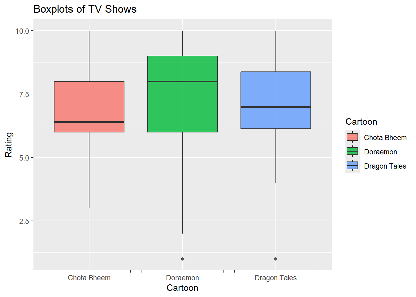
gf_boxplot(Rating ~ Cartoon, data = TV, fill =~Cartoon,alpha =0.8) %>%gf_vline(xintercept =~mean(Rating)) %>%gf_labs(title ="Boxplots of TV Shows",x ="Cartoon",y ="Rating") %>%gf_refine(scale_x_discrete(guide ="prism_bracket"), guides(fill =guide_legend(title ="Cartoon")))
Warning: The S3 guide system was deprecated in ggplot2 3.5.0.
ℹ It has been replaced by a ggproto system that can be extended.
From the analysis of cartoon ratings, it can be understood that Doraemon is the most liked and popular cartoon among the sample, as indicated by its highest median rating of 8.0 and an average rating of 7.2. The smaller IQR of about 1.5 suggests that viewers rate Doraemon consistently, indicating a strong and stable preference across the audience. Although there is one outlier (a much lower rating) most viewers rate it positively, confirming its popularity.
In comparison, Dragon Tales and Chota Bheem have slightly lower ratings and more varied viewer opinions. Dragon Tales has a median rating of 7.0 and an average of 7.3, with an IQR of approximately 2, reflecting a broader spread in ratings but still generally favourable opinions. Chota Bheem, on the other hand, has the lowest median rating of 6.4 and an average of 6.7 with an IQR around 2.5. It has a more varying reviews and possibly only appeals to a specific age. Overall, the ratings show a clear ranking, with Doraemon leading, followed by Dragon Tales and Chota Bheem ranks towards the lower end of the viewer’s preference.
Data Dictionary
Quantitative Variables
Rating: The numeric value or score given to each TV show based on likeness.
Qualitative Variables
Gender: Indicates the gender of individuals.
Cartoon: Represents the name of each TV show considered.
Statistical Analysis
Histogram
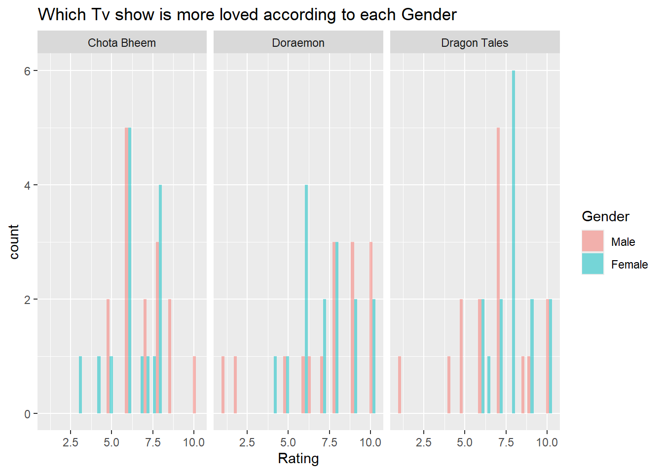
gf_histogram(~Rating, fill =~Gender,data = TV, alpha =0.5, position ="dodge") %>%gf_facet_wrap(vars(Cartoon)) %>%gf_labs(title="Which Tv show is more loved according to each Gender")
The histogram analysis reveals distinct gender-based preferences for each cartoon. Doraemon is popular across both boys and girls, with most ratings clustered around 7 to 8, indicating that it is consistently liked by both genders. In contrast, Dragon Tales seems to be more favored by girls, as their ratings peak around 10, while boys’ ratings are more clustered around 5 and 7. Chota Bheem, however, shows more varied opinions, where boys generally rate it lower, with a peak around 6, whereas girls have a wider range of ratings, peaking at around 6 but varying from from 5 till 10. Overall, Doraemon has broad appeal, Dragon Tales is especially popular among girls, and Chota Bheem receives more mixed reviews, with boys being less enthusiastic about it.
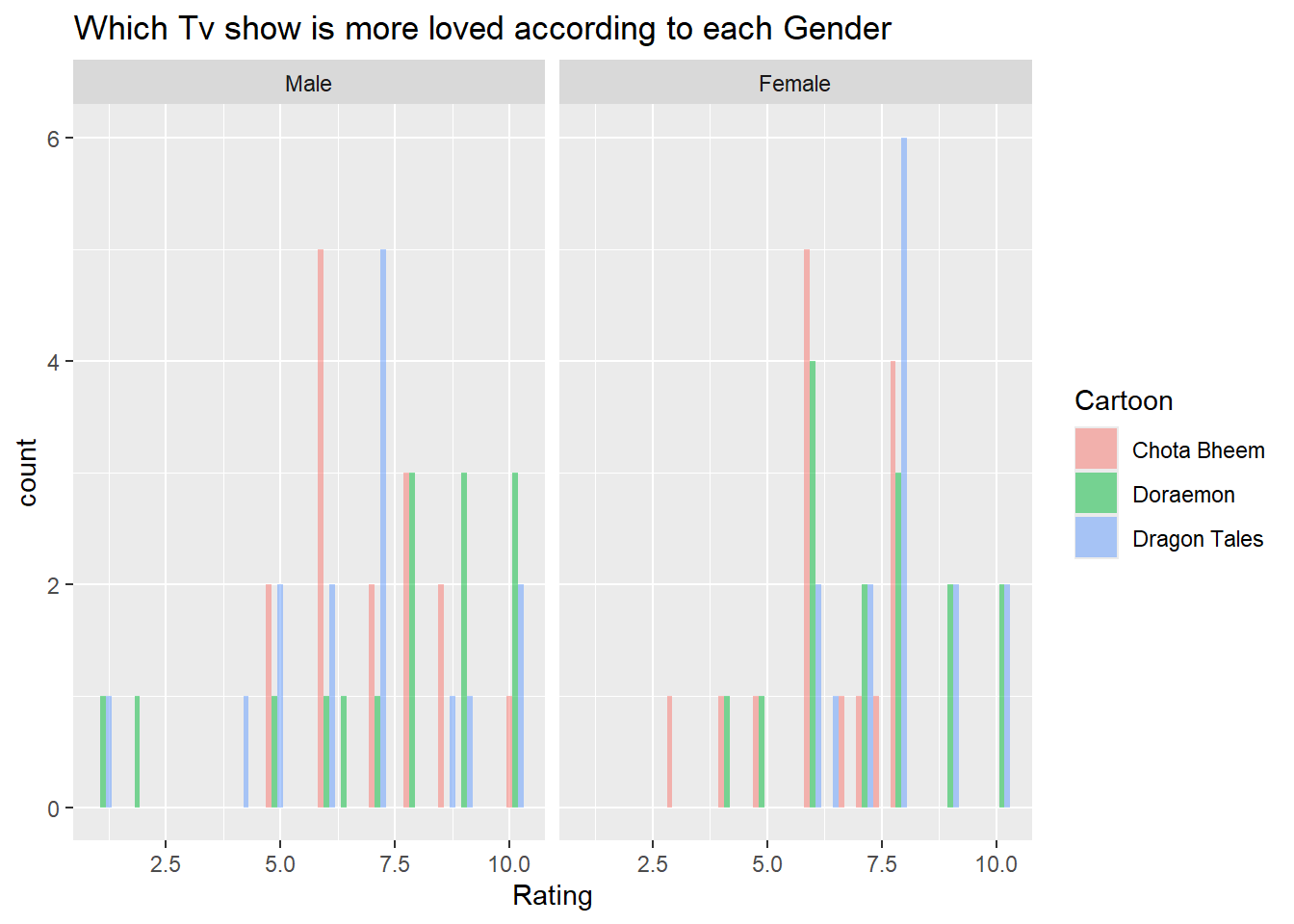
gf_histogram(~Rating, fill =~Cartoon,data = TV, alpha =0.5, position ="dodge") %>%gf_facet_wrap(vars(Gender)) %>%gf_labs(title="Which Tv show is more loved according to each Gender")
From this version, it is seen that boys tend to favor Doraemon, with ratings around 7 to 8, while Chota Bheem is rated lower, mostly around 5. However, girls rate Dragon Tales the highest, with peaks at 7 and 10, showing its popularity among them. This once again shows that Doraemon is the most universally liked, Dragon Tales is popular with girls, while Chota Bheem has more mixed ratings, especially among boys.
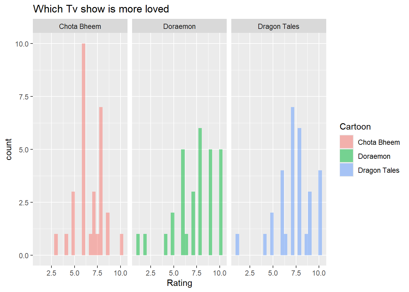
gf_histogram(~Rating, fill =~Cartoon,data = TV, alpha =0.5) %>%gf_facet_wrap(vars(Cartoon)) %>%gf_labs(title="Which Tv show is more loved")
The plot shows the distinct rating patterns of each cartoon. Doraemon stands out with ratings in the higher range, indicating it is consistently well-liked by viewers, with most ratings above 7. This high concentration reflects Doraemon’s stable popularity and little variation in how it’s rated.
Dragon Tales has a broader spread of ratings than Doraemon, with many viewers rating it between 7 and 10 but showing fewer perfect scores of 10. This indicates a wider variation in opinions, as most ratings cluster around 7. This indicates that its appeals to a diverse audience but lacks the same level of universally high approval.
Chota Bheem shows most ratings concentrated around the mid-range, primarily between 5 and 7. This lower score cluster indicates that Chota Bheem is less favored overall, with a stable but more moderate fan base. The narrow range of ratings suggests few viewers rate it exceptionally high or low, highlighting its limited but steady appeal compared to the other two cartoons.
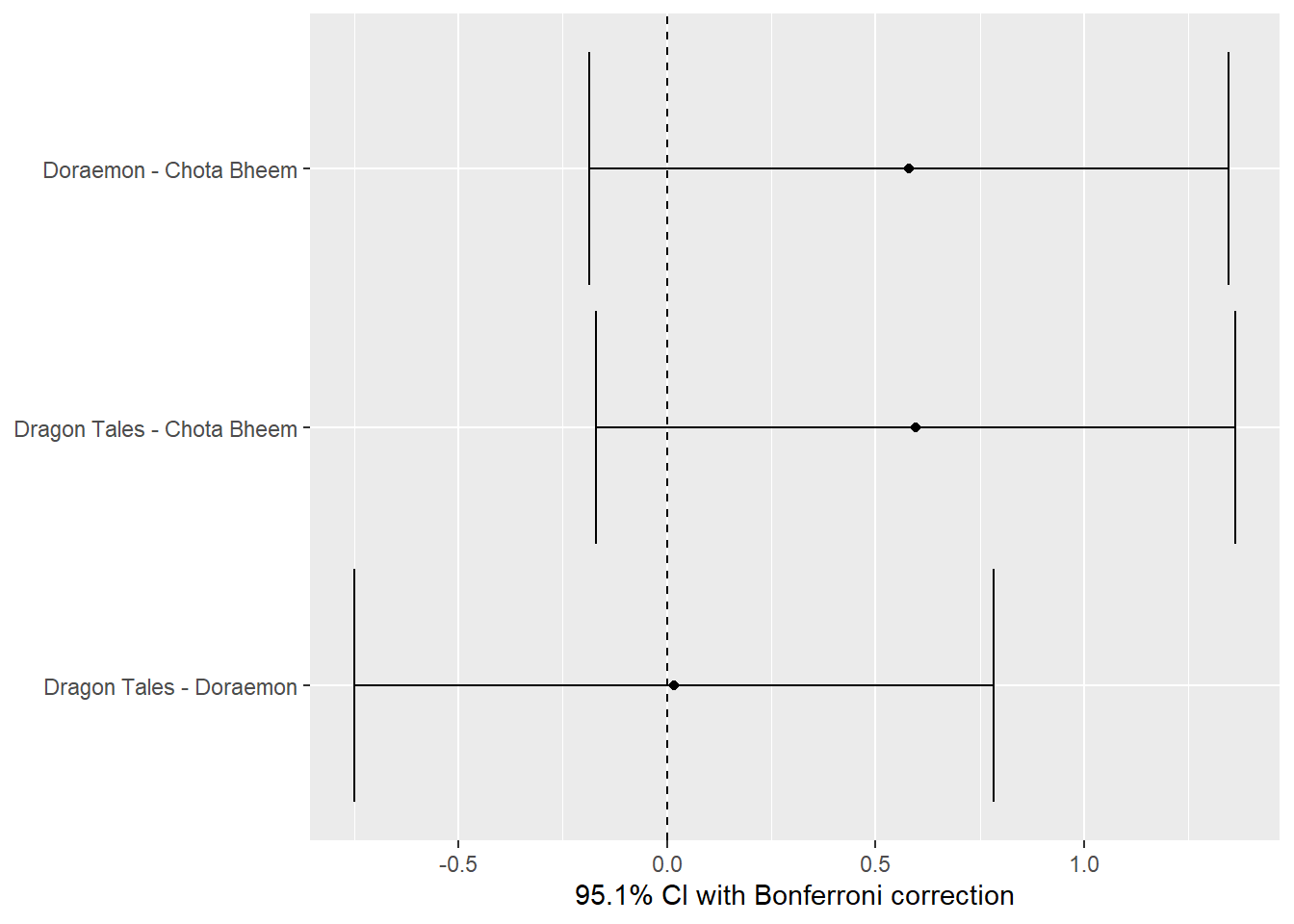
The plot includes 95.1% confidence intervals, adjusted for multiple comparisons using the Bonferroni correction. Each line represents the difference in ratings between two shows, with the dots indicating the average difference, and the horizontal lines showing the confidence intervals. Since all the confidence intervals cross zero, it shows that there is no statistically difference in the average ratings between the shows meaning that they were simply due to chance. The family-wise error rate of 0.049 means that, across all pairwise comparisons, the overall chance of incorrectly identifying a difference is 4.9%. However, in this analysis, no significant differences were detected.
The pairwise table again provides a result of no statistically significant differences in the average ratings. Although there are small differences in the mean ratings like a difference of 0.58 between Doraemon and Chota Bheem and 0.597 between Dragon Tales and Chota Bheem, the CI for each comparison includes zero, indicating that these differences are not statistically. Furthermore, the adjusted p-values are all above the typical significance threshold of 0.05, indicating that any observed differences are likely due to random chance. In summary, while there may be slight rating differences, they are not statistically significant, implying that viewers’ ratings for these cartoons are generally similar when accounting for multiple comparisons.
Effect Size
TV_aov
Call:
   aov(formula = Rating ~ Cartoon, data = TV)

Terms:
                 Cartoon Residuals
Sum of Squares    6.9269  327.9047
Deg. of Freedom        2        87

Residual standard error: 1.941396
Estimated effects may be unbalanced
The analysis shows that the Cartoon factor has a sum of squares of 6.9269, while the sum of squares for the Residuals is 327.9047. This indicates that most of the variability in ratings is due to the residuals, meaning that differences in ratings between the cartoons are not large compared to the overall differences in the data. The degrees of freedom (indicates the number of groups for a factor minus one), for the Cartoon factor is 2 meaning that there are three groups being compared.
The residual standard error is 1.941396 indicates that, on average the ratings deviate by about 1.94 points from their respective group averages. This means that while the average ratings have a central value for each cartoon, the actual ratings can vary around this average.
Overall, while there are some differences in ratings among the cartoons, they are relatively small compared to the overall variation in the data, indicating that the differences in ratings may not be important.
Null Hypothesis
There is no difference in ratings for the various TV shows.
Checking ANOVA Assumptions
Data and errors are normally distributed.
Variances are equal.
Observations are independent.
Shapiro Test
shapiro.test(x = TV$Rating)
    Shapiro-Wilk normality test

data:  TV$Rating
W = 0.93517, p-value = 0.0002269
The Shapiro test has a p-value of 0.0002269 indicating that it does follow normal distribution since it much smaller than 0.05. It also means that the ratings are skewed and as a result using statistical methods that assume normality cannot be used for further analysis.
The results of the Shapiro test for the ratings grouped by cartoon show different values for normality. For Chota Bheem, the p-value is 0.18538322, indicating that the distribution is normal as the value is more than 0.05.
Whereas, both Doraemon and Dragon Tales have much lower p-values at 0.01385422 and 0.02395200 respectively. This indicates that the ratings for these cartoons do not follow a normal distribution. This lack of normality may limit the reliability of statistical analyses conducted on these ratings, which is when alternative methods are used to ensure accurate conclusions.
Residual-Post Model
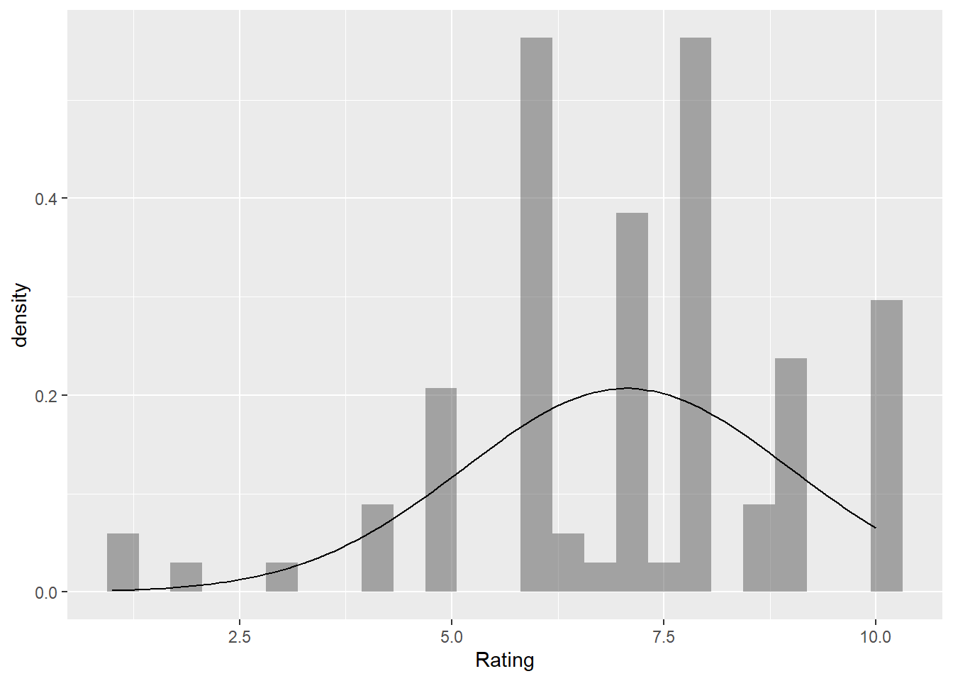
TV %>%as_tibble() %>%gf_dhistogram(~Rating, data = .) %>%gf_fitdistr(dist ="dnorm")
##TV %>%as_tibble() %>%gf_qq(~Rating, data = .) %>%gf_qqstep() %>%gf_qqline()
##shapiro.test(TV_aov$residuals)
    Shapiro-Wilk normality test

data:  TV_aov$residuals
W = 0.93926, p-value = 0.0003856
The histogram of the ratings in the TV dataset reveals a leftward skew, with the frequency of different rating values showing that there are more ratings concentrated at the higher end, around 8, after which it starts reducing as the values approach 10. This skewness indicates that the ratings do not follow normal distribution. The fitted normal distribution drawn on the histogram clearly shows the difference between the actual ratings and what a normal distribution would look like. This reconfirms the observation that the ratings are not normally distributed.
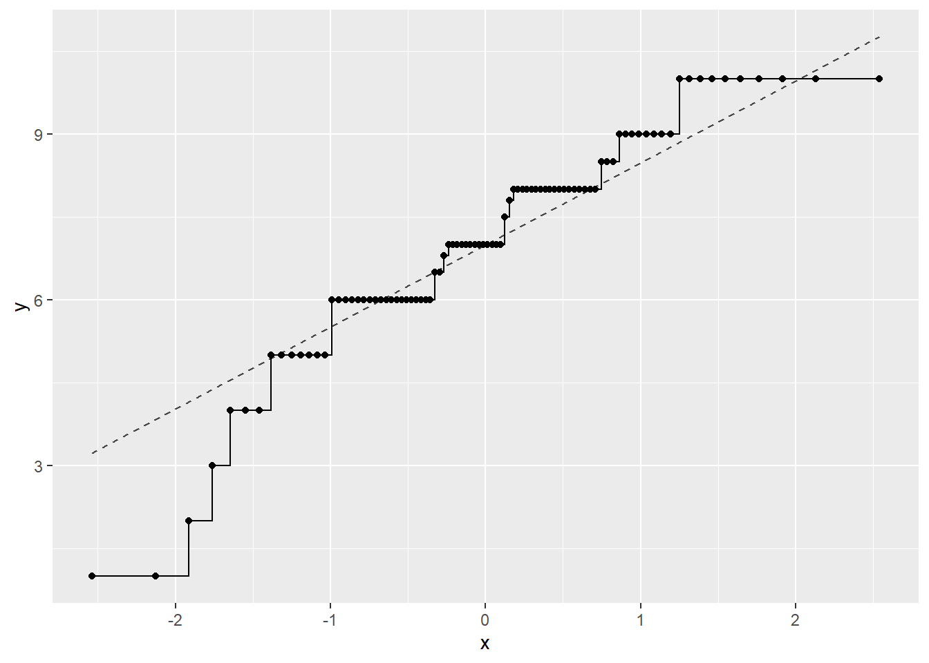
The Q-Q plot or Quantile-Quantile plot or Probability plot compares the quantiles of a dataset to the quantiles of a normal distribution, similar to the quartiles used in box plots. In the Q-Q plot for the ratings, the points represent the quantiles of the ratings plotted against the quantiles of a normal distribution. The results show that most points do not follow the reference line, indicating that the ratings are not normally distributed, as the majority of points fall below the line, further confirming the findings from the histogram analysis.
The Shapiro test for residuals from the ANOVA analysis show a p-value of 0.0003856, indicating a strong rejection of the null hypothesis of normality. This implies that the residuals exhibit significant departures from normality.
# A tibble: 2 × 2
  Gender variance
  <fct>     <dbl>
1 Male       4.92
2 Female     2.66
DescTools::LeveneTest(Rating ~ Cartoon, data = TV)
Levene's Test for Homogeneity of Variance (center = median)
      Df F value Pr(>F)
group  2  1.2923 0.2798
      87
fligner.test(Rating ~ Cartoon, data = TV)
    Fligner-Killeen test of homogeneity of variances

data:  Rating by Cartoon
Fligner-Killeen:med chi-squared = 1.8135, df = 2, p-value = 0.4038
The analysis of variance for the ratings based on gender showed the variance for each group. Levene’s Test for Homogeneity of Variance indicated that there is no significant difference in the variances of the ratings among the three cartoons, with a p-value of 0.2798. This means that the ratings across groups are similar. Similarly, the Fligner-Killeen test also showed no significant differences in variances, with a chi-squared value of 1.8135 and a p-value of 0.4038. Both tests suggest that the assumption of equal variances across the groups is met, which is an important condition for conducting further statistical analyses.
The chi-square statistic is calculated by summing the squared differences between observed and expected frequencies, divided by the expected frequencies for each category. A higher chi-square value indicates a greater discrepancy between observed and expected values. The result is then compared to a critical value from the chi-square distribution to assess statistical significance, which depends on the degrees of freedom associated with the test.
Response: Rating (numeric)
Explanatory: Cartoon (factor)
Null Hypothesis: independence
# A tibble: 1 × 1
   stat
  <dbl>
1 0.919
It shows that the F statistic value of 0.9189 is the ratio of variance between the cartoons to the variance within the groups. A lower F value indicates that the differences in ratings among the cartoons are minimal compared to the differences in ratings within each cartoon group. This result reconfirms previous findings of no significant differences in the average ratings among the cartoons.
null_dist_infer <- TV %>%specify(Rating~Cartoon) %>%hypothesise(null ="independence") %>%generate(reps =4999, type ="permute") %>%calculate(stat ="F")##null_dist_infer
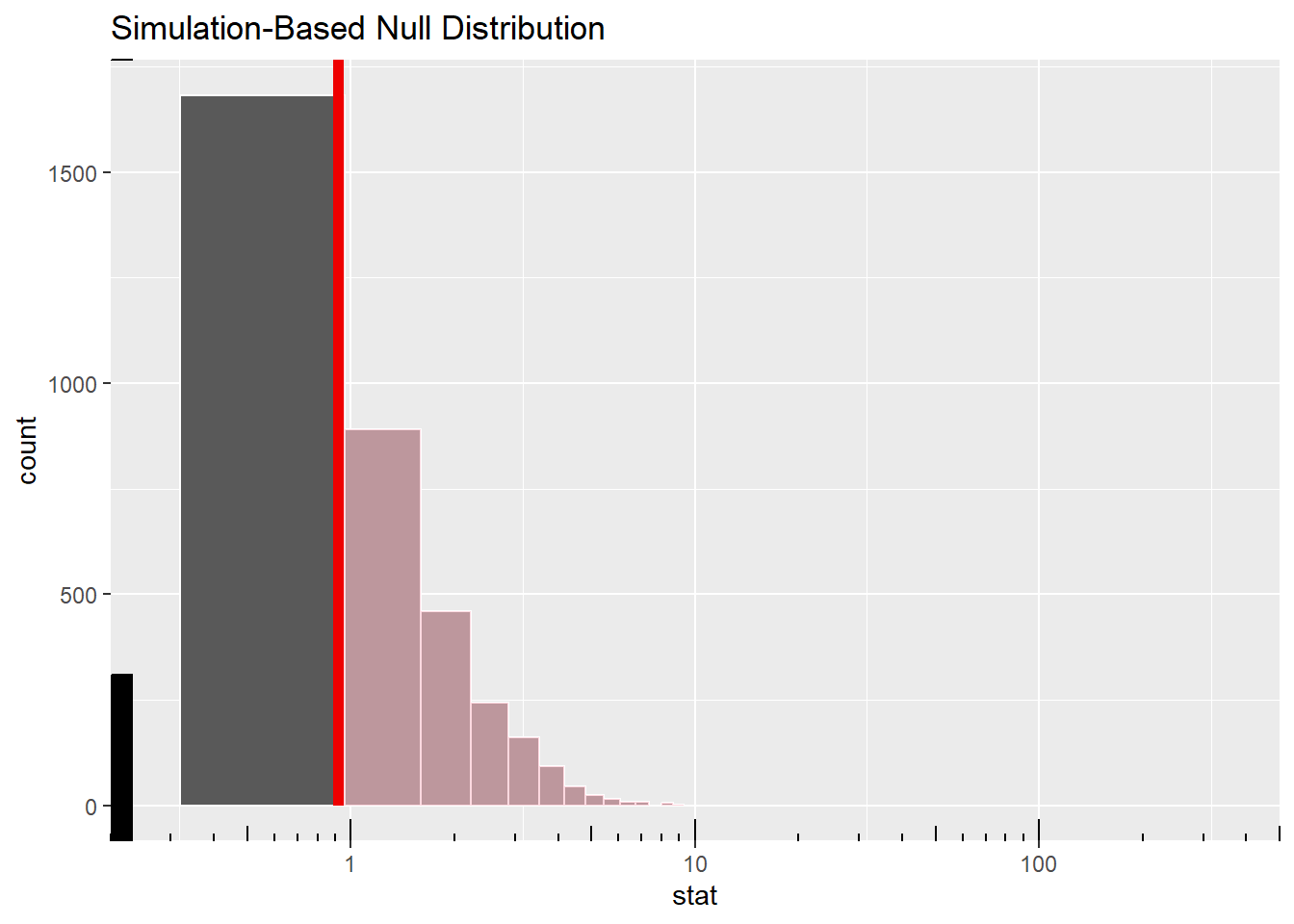
The plot illustrates the range of F values observed under the null hypothesis of independence, which assumes no true differences in ratings among the cartoons. The observed F statistic is 0.9189, falling within the null distribution of the 4999 times shuffled F statistic. The shaded area to the right indicates how likely it is to get an F statistic that is greater than the observed value of 0.9189 if the null hypothesis is true. In hypothesis testing, the null hypothesis usually states that there is no difference between groups.
The range of values in the null distribution extends from about 0.00011 to over 10.5. Given that the observed F statistic is low in comparison to the values in the null distribution, it indicates a high likelihood of obtaining a statistic if the null hypothesis is true. This suggests insufficient evidence to reject the null hypothesis, confirming the conclusion that the average ratings for the cartoons are likely similar and any observed differences are likely due to random chance.
The red line falling just before 1 further supports this conclusion, indicating that the variance between the cartoon groups is not significantly greater than the variance within the groups, which again confirms that there are no significant differences in average ratings among the cartoons.
Conclusion
In this analysis of the ratings for three children’s TV shows “Doraemon, Dragon Tales, and Chota Bheem” various statistical tests including ANOVA, Shapiro tests, and permutation tests, were used to explore differences in viewer preferences. The ANOVA results indicated that there were no statistically significant differences in average ratings among the three cartoons, as shown by the F statistic of 0.9189. This indicates that any variations in ratings are likely due to random chance.
The Shapiro test revealed that the ratings for Doraemon and Dragon Tales were not normally distributed, while Chota Bheem’s ratings appeared to follow a normal distribution. Additionally, Levene’s test confirmed that the assumption of equal variances across the groups was met, indicating that the spread of ratings for each cartoon was similar. An error plot also showed the differences and uncertainty in ratings across the cartoons, with confidence intervals indicating the range of viewer preferences for each show. This further showed that while Doraemon had the highest ratings, the overlaps in confidence intervals among the three cartoons suggest that the differences in viewer preferences are not statistically significant.
The boxplots demonstrated that Doraemon received the highest median rating of 8.0, with a consistent spread among viewers. In contrast, Dragon Tales had a median rating of 7.0 with greater variation, while Chota Bheem was at the end with a median rating of 6.4 and a wider range in opinions. Histograms indicated that Doraemon was generally favored by both genders, whereas Dragon Tales showed a peak in ratings among girls, and Chota Bheem received more mixed reviews, particularly from boys.
Overall, the findings suggest that while Doraemon stands out as the most popular cartoon among college students, the differences in ratings between the shows are not statistically significant. This implies that all three cartoons have a reasonable level of likeness, though preferences vary by gender and specific audiences. The combination of statistical tests and visual representations also shows that the ratings reflect subjective tastes rather than high differences in quality or appeal.