Differences in Tips from Vegetarians ans Non-Vegetarians
Differences in Tips from Vegetarians ans Non-Vegetarians
Author
Sara S
Introduction
The case study named “I will eat my tip, thank you” is an exploration of difference in tips given by vegetarians and non-vegetarians in the student population. The sample population considered and used for the dataset are students from the various MAHE colleges with equal number of women and men.
Importing Packages
library(tidyverse)
── Attaching core tidyverse packages ──────────────────────── tidyverse 2.0.0 ──
✔ dplyr     1.1.4     ✔ readr     2.1.5
✔ forcats   1.0.0     ✔ stringr   1.5.1
✔ ggplot2   3.5.1     ✔ tibble    3.2.1
✔ lubridate 1.9.3     ✔ tidyr     1.3.1
✔ purrr     1.0.2
── Conflicts ────────────────────────────────────────── tidyverse_conflicts() ──
✖ dplyr::filter() masks stats::filter()
✖ dplyr::lag()    masks stats::lag()
ℹ Use the conflicted package (<http://conflicted.r-lib.org/>) to force all conflicts to become errors
library(ggformula)
Loading required package: scales

Attaching package: 'scales'

The following object is masked from 'package:purrr':

    discard

The following object is masked from 'package:readr':

    col_factor

Loading required package: ggridges

New to ggformula?  Try the tutorials:
    learnr::run_tutorial("introduction", package = "ggformula")
    learnr::run_tutorial("refining", package = "ggformula")
library(mosaic)
Registered S3 method overwritten by 'mosaic':
  method                           from
  fortify.SpatialPolygonsDataFrame ggplot2

The 'mosaic' package masks several functions from core packages in order to add
additional features.  The original behavior of these functions should not be affected by this.

Attaching package: 'mosaic'

The following object is masked from 'package:Matrix':

    mean

The following object is masked from 'package:scales':

    rescale

The following objects are masked from 'package:dplyr':

    count, do, tally

The following object is masked from 'package:purrr':

    cross

The following object is masked from 'package:ggplot2':

    stat

The following objects are masked from 'package:stats':

    binom.test, cor, cor.test, cov, fivenum, IQR, median, prop.test,
    quantile, sd, t.test, var

The following objects are masked from 'package:base':

    max, mean, min, prod, range, sample, sum
library(broom)library(infer)
Attaching package: 'infer'

The following objects are masked from 'package:mosaic':

    prop_test, t_test
library(nortest)library(dplyr)library(crosstable)
Attaching package: 'crosstable'

The following object is masked from 'package:purrr':

    compact
Dataset: Tip
tip <-read_csv("../../data/tip.csv")
Rows: 60 Columns: 4
── Column specification ────────────────────────────────────────────────────────
Delimiter: ","
chr (3): Name, Gender, Preferance
dbl (1): Tip

ℹ Use `spec()` to retrieve the full column specification for this data.
ℹ Specify the column types or set `show_col_types = FALSE` to quiet this message.
tip
# A tibble: 60 × 4
   Name     Gender Preferance   Tip
   <chr>    <chr>  <chr>      <dbl>
 1 Aanya    Female Veg            0
 2 Adit     Male   Veg            0
 3 Aditi    Female Veg           20
 4 Akash    Male   Non-veg        0
 5 Akshita  Female Non-veg        0
 6 Anandita Female Non-veg        0
 7 Ananya   Female Non-veg       20
 8 Anaya    Female Veg           35
 9 Anhuya   Female Veg           40
10 Ankit    Male   Non-veg        0
# ℹ 50 more rows
categorical variables:
        name     class levels  n missing
1       Name character     60 60       0
2     Gender character      2 60       0
3 Preferance character      2 60       0
                                   distribution
1 Aanya (1.7%), Adit (1.7%) ...
2 Female (50%), Male (50%)
3 Non-veg (50%), Veg (50%)

quantitative variables:
  name   class min Q1 median Q3 max     mean       sd  n missing
1  Tip numeric   0  0      0 20 100 11.16667 17.83556 60       0
Factorizing the data
tip2 <- tip %>%mutate(Preferance =as_factor(Preferance),Gender =as_factor(Gender) )tip2
# A tibble: 60 × 4
   Name     Gender Preferance   Tip
   <chr>    <fct>  <fct>      <dbl>
 1 Aanya    Female Veg            0
 2 Adit     Male   Veg            0
 3 Aditi    Female Veg           20
 4 Akash    Male   Non-veg        0
 5 Akshita  Female Non-veg        0
 6 Anandita Female Non-veg        0
 7 Ananya   Female Non-veg       20
 8 Anaya    Female Veg           35
 9 Anhuya   Female Veg           40
10 Ankit    Male   Non-veg        0
# ℹ 50 more rows
categorical variables:
        name     class levels  n missing
1       Name character     60 60       0
2     Gender    factor      2 60       0
3 Preferance    factor      2 60       0
                                   distribution
1 Aanya (1.7%), Adit (1.7%) ...
2 Female (50%), Male (50%)
3 Veg (50%), Non-veg (50%)

quantitative variables:
  name   class min Q1 median Q3 max     mean       sd  n missing
1  Tip numeric   0  0      0 20 100 11.16667 17.83556 60       0
skimr::skim(tip2)
Data summary
Name
tip2
Number of rows
60
Number of columns
4
_______________________
Column type frequency:
character
1
factor
2
numeric
1
________________________
Group variables
None
Variable type: character
skim_variable
n_missing
complete_rate
min
max
empty
n_unique
whitespace
Name
0
1
4
9
0
60
0
Variable type: factor
skim_variable
n_missing
complete_rate
ordered
n_unique
top_counts
Gender
0
1
FALSE
2
Fem: 30, Mal: 30
Preferance
0
1
FALSE
2
Veg: 30, Non: 30
Variable type: numeric
skim_variable
n_missing
complete_rate
mean
sd
p0
p25
p50
p75
p100
hist
Tip
0
1
11.17
17.84
0
0
0
20
100
▇▁▁▁▁
Data Dictionary
Quantitative Variables
Tip: A numerical variable that represents the amount of tip given.
###Qualitative Variables Gender: Indicates the gender of individuals. Preference: Indicates dietary preference (Veg or Non-veg).
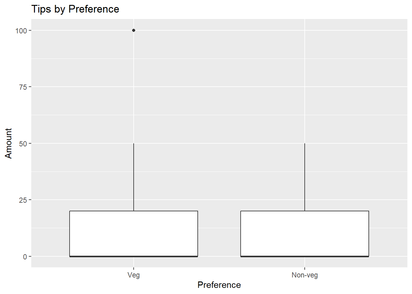
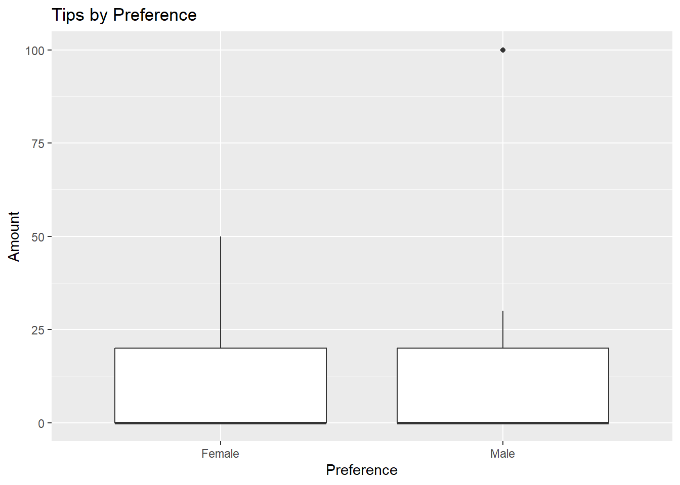
gf_boxplot(Tip ~ Preferance, data = tip2) %>%gf_labs(title ="Tips by Preference",x ="Preference",y ="Amount" )
The tipping behavior between vegetarian and non-vegetarian groups shows a slight difference in the mean value, with vegetarians averaging a mean tip of 12.3 (with a standard deviation of 21.9) compared to 10.0 for non-vegetarians (with a standard deviation of 12.9). The minimum and maximum tips for vegetarians range from 0 to 100, while non-vegetarians only go up to 50. The plot indicates the presence of an outlier in the vegetarian group, with a single individual tipping 100, which significantly exceeds the other amounts. Both groups exhibit a median tip of 0, suggesting that most people either do not tip or tip very minimally. Overall, this analysis indicates that while there are a few instances of higher tips among vegetarians, tip amounts are generally low across both groups, with only a few individuals tipping at higher levels.
Mean and Standard Deviation for Tip
tip_mean <- mosaic::mean(~Tip, data = tip2)tip_sd <- mosaic::sd(~Tip, data = tip2)tip_mean
[1] 11.16667
tip_sd
[1] 17.83556
Preference
Histogram
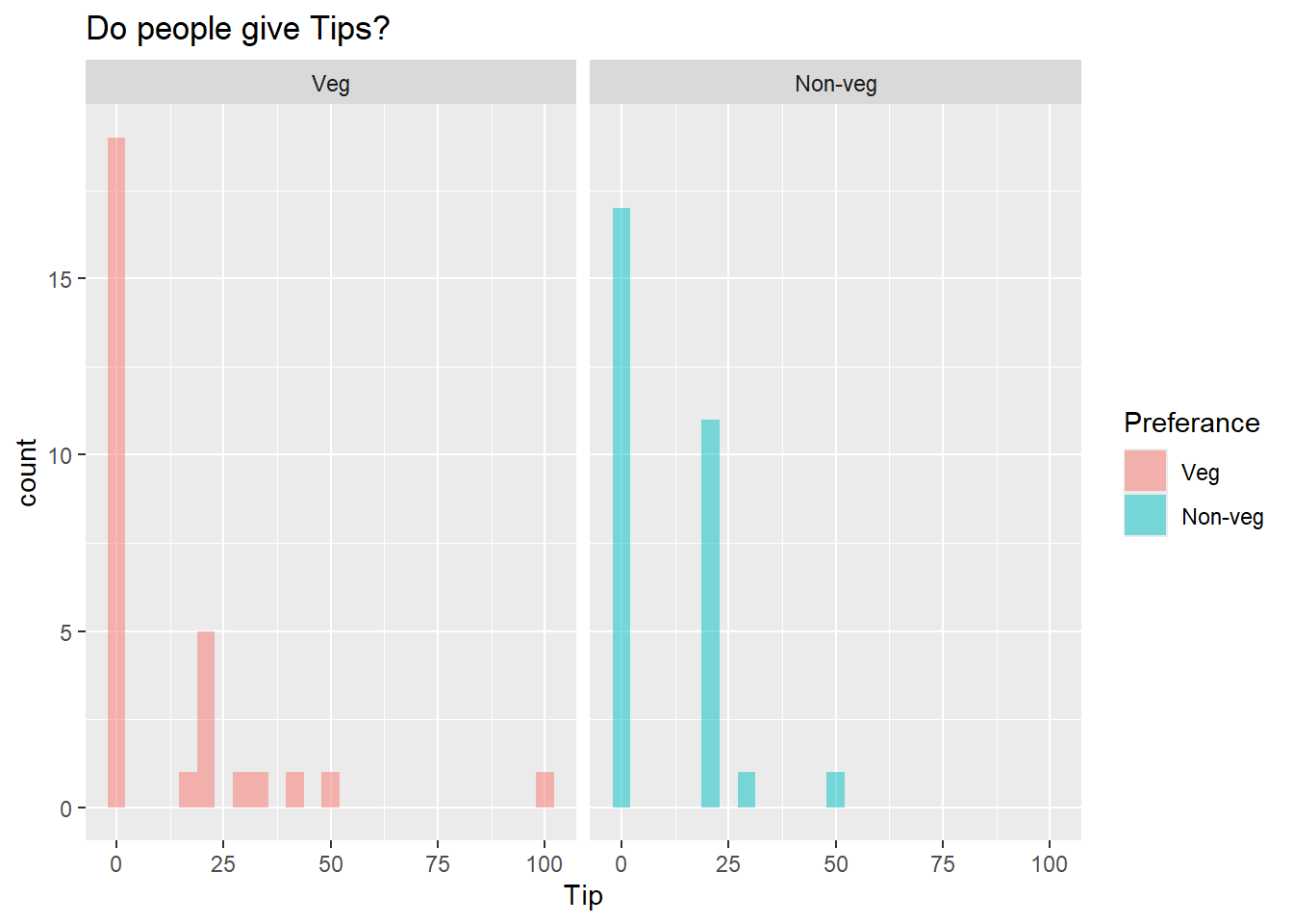
gf_histogram(~Tip,fill =~Preferance, data=tip2)%>%gf_facet_wrap(vars(Preferance)) %>%gf_labs(title="Do people give Tips?")
Both groups display a higher concentration of tips towards the lower end of the scale, with most individuals tipping between 0 and 20. The vegetarian group shows a wider range of tipping behavior, with a few individuals giving significantly higher amounts. While the non-vegetarians have similar and lower tips, showing a more consistent tipping behavior among them. There are fewer high-value tips in the non-vegetarian group, proving once again that many non-vegetarians either do not tip or typically give minimal amounts. Although there are some differences in tipping patterns between the two groups, overall, tips remain low across both categories, with a significant number of individuals giving no tips at all.
Null Hypothesis
There is no significant difference in tipping behavior between non-vegetarian and vegetarian individuals.
Density graph
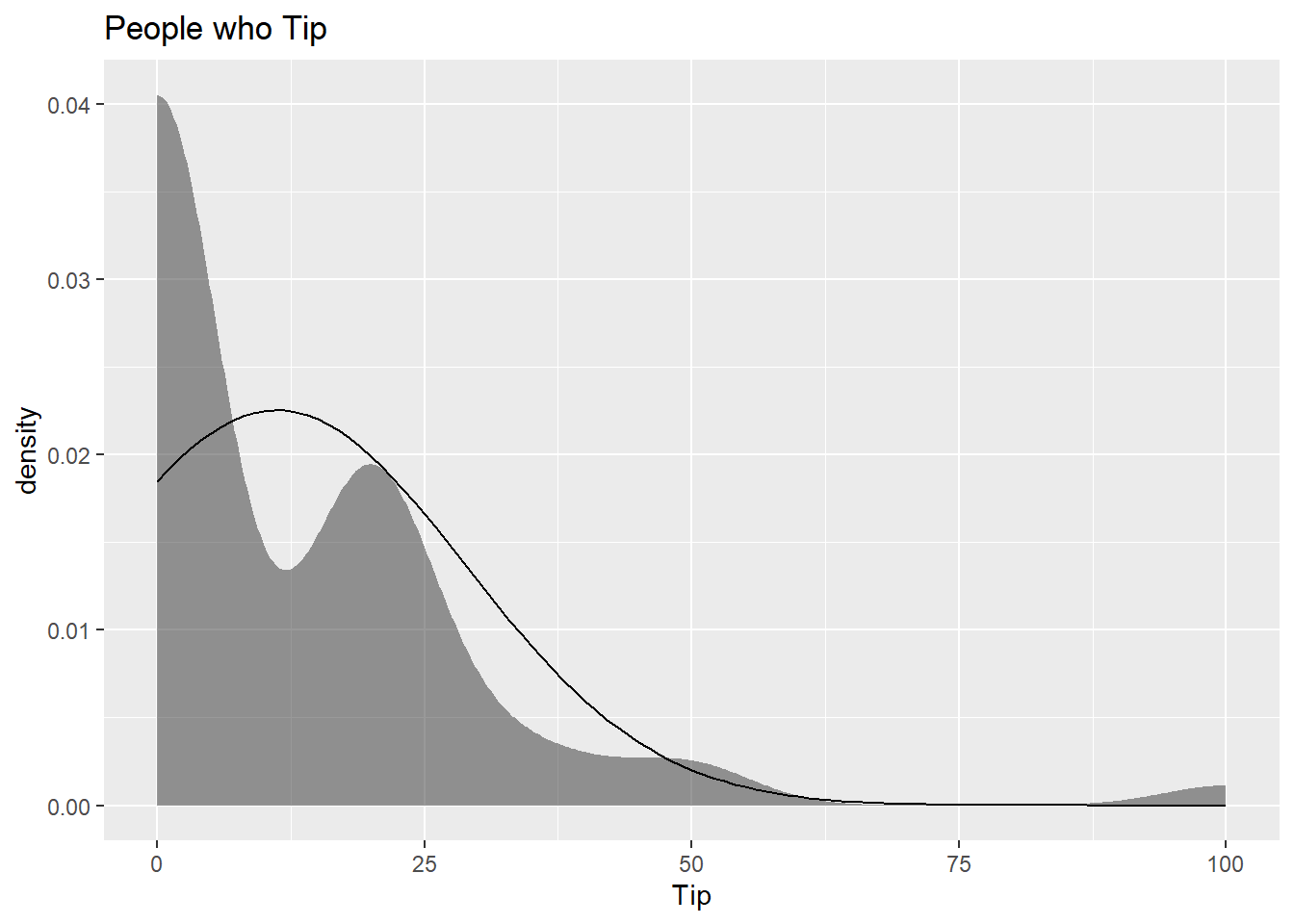
tip2 %>%gf_density(~Tip, title="People who Tip")%>%gf_fitdistr(dist="dnorm")
The plot shows a noticeable peak at the lower end of the tipping scale, indicating that most individuals tend to tip minimal amounts, particularly around 0 to 20. The distribution gradually decreases as tip amounts increase, suggesting that higher tips are less common. The line for the normal distribution confirms that the majority of tips are concentrated in the lower range, emphasizing the idea that tipping is generally low among the student population.
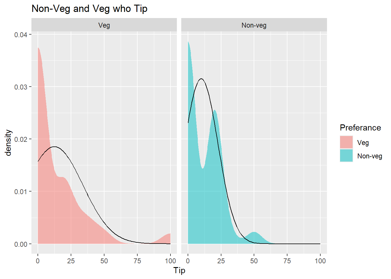
tip2 %>%gf_density(~Tip, fill=~Preferance, alpha=0.5, title="Non-Veg and Veg who Tip")%>%gf_facet_grid(~Preferance) %>%gf_fitdistr(dist="dnorm")
Both groups show a peak at the lower end of the tipping scale, with most tips from 0 to around 10 for vegetarians and to around 20 for non-vegetarians. However, the veg group exhibit a slightly wider spread, with a few tipping significantly higher amounts compared to non-vegetarians, who consistently tip at lower amounts. The normal distribution lines for each group reveals that while both distributions are skewed towards lower tips, the vegetarian group demonstrates more variation, highlighting differences in tipping behavior between the two dietary preferences.
The test statistic is 0.50, with a p-value of 0.62, indicating no statistically significant difference in tipping behavior between the two groups. The confidence interval ranges from about -6.99 to 11.66, suggesting that the true difference in average tips could fall anywhere within this range. Since the p-value is much higher 0.05, it means there isn’t enough evidence to reject the null hypothesis, implying that tipping patterns between vegetarians and non-vegetarians are similar.
    Shapiro-Wilk normality test

data:  NV$Tip
W = 0.71661, p-value = 2.747e-06
shapiro.test(V$Tip)
    Shapiro-Wilk normality test

data:  V$Tip
W = 0.6286, p-value = 1.661e-07
The Shapiro normality test results for the tipping data show that both non-vegetarians and vegetarians do not follow a normal distribution. For the non-vegetarian group, the test produced a p-value of 2.747e-06 (2.747× 10 to the power negative 6 = 0.000002747), while the vegetarian group had a p-value of 1.661e-07 (1.6617× 10 to the power negative 7 = 0.0000001661). Since both p-values are significantly lower than 0.05, the null hypothesis of normality is rejected for both groups. This indicates that the tipping behavior in both categories is not normally distributed, suggesting that non-parametric methods need to be used for further analysis.
Non-parametric methods are statistical techniques that do not assume a specific distribution for the data, making them useful when the data doesn’t follow a normal distribution. Eg: Wilcoxon test
Parametric methods are statistical techniques that assume the data follows a specific distribution, typically a normal distribution. Eg:T-test and ANOVA
Wilcoxon Test
wilcox.test(Tip ~ Preferance, data = tip2,conf.int =TRUE,conf.level =0.95) %>% broom::tidy()
Warning in wilcox.test.default(x = DATA[[1L]], y = DATA[[2L]], ...): cannot
compute exact p-value with ties
Warning in wilcox.test.default(x = DATA[[1L]], y = DATA[[2L]], ...): cannot
compute exact confidence intervals with ties
The results from the Wilcoxon rank sum test indicates that there is no significant difference in tipping amounts between vegetarians and non-vegetarians.With a p-value of 0.8327, much higher than 0.05, it shows that the null hypothesis cannot be rejected, showing once again that the tipping behavior in both groups is similar.
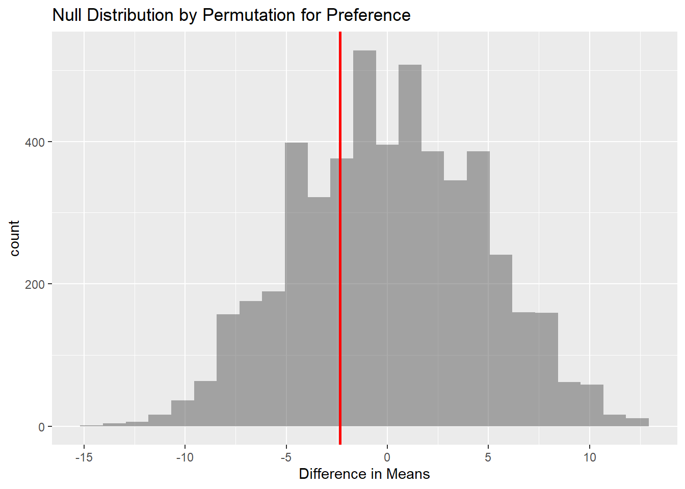
Permutation
obs_mean <-diffmean(Tip~Preferance, data = tip2)obs_mean
 diffmean
-2.333333
null_dist <-do(4999) *diffmean(data = tip2, Tip ~shuffle(Preferance))null_dist
gf_histogram(data = null_dist, ~ diffmean, bins =25) %>%gf_vline(xintercept = obs_mean, colour ="red", linewidth =1,title ="Null Distribution by Permutation for Preference") %>%gf_labs(x ="Difference in Means")
The permutation test is conducted to analyze the difference in tipping amounts between vegetarians and non-vegetarians without checking for normality or other assumptions, simply by shuffling the data between the groups. The observed mean difference in tips is calculated to be -2.333333, indicating that, on average, vegetarians tip less than non-vegetarians. To better this difference, a null distribution is generated by shuffling the ‘Preferance’ variable 4999 times, allowing for the comparison of the observed mean difference against this distribution. The proportion of the null distribution that is less than or equal to the observed mean difference is then calculated and visualized via a histogram with 25 bins. A red vertical line that marks the position of the observed mean difference. This visualization helps to determine if the observed difference is likely due to random chance and this plot has a central placement indicating that the observed difference may be due to chance. Once again showing that vegetarians and non-vegetarians tip similarly.
Gender
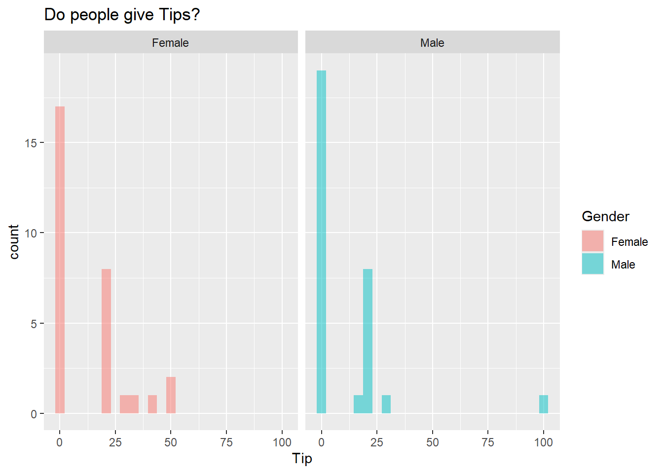
gf_histogram(~Tip,fill =~Gender, data=tip2)%>%gf_facet_wrap(vars(Gender)) %>%gf_labs(title="Do people give Tips?")
gf_boxplot(Tip ~ Gender, data = tip2) %>%gf_labs(title ="Tips by Preference",x ="Preference",y ="Amount" )
Both males and females mostly tip low amounts, with most people giving tips between 0 and 20. However, females have a wider variety in their tipping, with some tipping much higher than others, showing a few noticeable outliers. On the other hand, males usually tip lower amounts more consistently, with only a few higher tips, notably one at 100 from a vegetarian. Overall, the data shows that while both genders usually tip low, females tend to have more differences in their tipping amounts compared to males.
Null Hypothesis
There is no difference between tips for male and female
Density Graph
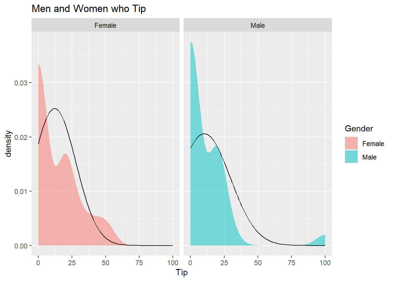
tip2 %>%gf_density(~Tip, fill=~Gender, alpha=0.5, title="Men and Women who Tip")%>%gf_facet_grid(~Gender) %>%gf_fitdistr(dist="dnorm")
The fitted normal distribution lines indicate that while tipping is generally low for both men and women, mostly between 0 and 20, women’s tipping behavior shows more variability, with some individuals tipping significantly higher. This finding aligns with density plot of the actual population and reconfirms the insights gathered from the histogram.
The t-test shows that the mean tip for women is 12.17, while for men it is 10.17. The p-value is 0.67 indicating that there is no statistically significant difference in the tipping behavior between the two genders. The confidence interval for the mean difference ranges from -7.29 to 11.29, suggesting that the true difference in mean tips could be negative or positive, further showing the lack of significant difference in tipping patterns between men and women.
    Shapiro-Wilk normality test

data:  FM$Tip
W = 0.74757, p-value = 8.321e-06
shapiro.test(M$Tip)
    Shapiro-Wilk normality test

data:  M$Tip
W = 0.53209, p-value = 1.19e-08
The results of the Shapiro test indicate that the tipping data for both females and males does not follow a normal distribution. For the female group, the test produced a p-value of approximately 0.00000832, while for the male group, the p-value was about 0.000000012. Since both p-values are significantly lower than 0.05, this leads to the rejection of the null hypothesis of normality for both genders. This suggests that the tipping behavior for both females and males is not normally distributed, which is why non-parametric tests needs to be conducted for further analysis.
Wilcox Test
wilcox.test(Tip ~ Gender, data = tip2,conf.int =TRUE,conf.level =0.95) %>% broom::tidy()
Warning in wilcox.test.default(x = DATA[[1L]], y = DATA[[2L]], ...): cannot
compute exact p-value with ties
Warning in wilcox.test.default(x = DATA[[1L]], y = DATA[[2L]], ...): cannot
compute exact confidence intervals with ties
The estimated difference in tips is approximately 0.00004446, with a p-value of 0.42207. Since the p-value is greater than 0.05, it suggests that there is no difference in tipping amounts between genders. The confidence interval ranges from -0.00001344 to 0.00000497, indicating that any differences in tipping behavior between the two groups are minimal and not statistically significant.
Permutation
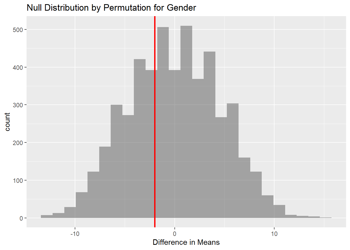
obs_mean1 <-diffmean(Tip~Gender, data = tip2)obs_mean1
diffmean
      -2
null_dist2 <-do(4999) *diffmean(data = tip2, Tip ~shuffle(Gender))null_dist2
###prop1(~ diffmean <= obs_mean1, data = null_dist2)
prop_TRUE
   0.3632
###gf_histogram(data = null_dist2, ~ diffmean, bins =25) %>%gf_vline(xintercept = obs_mean1, colour ="red", linewidth =1,title ="Null Distribution by Permutation for Gender") %>%gf_labs(x ="Difference in Means")
To determine if the difference in tipping between genders is statistically significant, a null distribution is created by randomly shuffling the Gender variable 4,999 times, allowing for a comparison with the observed mean difference of -2. The results show that about 35.84% of the null distribution. It shows how often the random shuffling resulted in a mean difference that is as extreme as the observed difference of -2. Since about 35.84% of the shuffled results are less than or equal to -2, it means there is a 35.84% chance that such a mean difference could occur by random, indicating that there may not be a real difference in tipping behavior between genders. The red line is the position of the observed mean difference. Overall, this plot shows that the observed difference falls within the range of what might occur by random chance, once again showing that the tipping behavior between genders is similar rather than significantly different.
Conclusion
This study examined the tipping behavior of vegetarians and non-vegetarians, as well as the differences in tips given by males and females among students. The initial analysis using a t-test indicated no significant difference in tipping amounts between the groups, with p-values above 0.05. However, since both groups’ tipping data did not follow a normal distribution, as confirmed by the Shapiro test, non-parametric methods like the Wilcoxon test were conducted for more reliable results. The Wilcoxon test further supported the findings of the t-test, showing no significant difference in tips between vegetarians and non-vegetarians, or between males and females. Additionally, the permutation test showed how often observed differences might occur due to random chance, reconfirming the findings that tipping behaviors are similar across the examined groups. Overall, the combination of these statistical tests provided a clear understanding of tipping behavior among students, revealing that tipping amounts were generally low, often reaching 0, across all analyzed groups.